A note on the series:

This post is part of a series of weekly discussion prompts for my class DSBA-6190: Introduction to Cloud Computing. Each prompt includes two or three general questions on a cloud computing related topic, along with screenshot from a interactive online lab.

How does the CAP Theorem play a role in designing for the cloud?

The CAP Theorem outlines the tradeoffs between three properties when developing a distributed system for storing data, of which any Cloud Computing application would apply. The three properties are:

• Consistency: All users must see the same information
• Availability: All users can access the data when needed
• Partitioning: The system has tolerance to network partitions (and network failures)

Any cloud system is going to be a collection of nodes synced horizontally. These nodes may be fairly cheap standard hardware, so many nodes may be required. Due to the size of these cloud systems, and the type of equipment that may be used, the need to cope with node failures is a given. In terms of CAP theorem, that means the cloud system must deal with Partitioning (P).

Therefore, the balancing act is between Consistency and Availability. In this trade-off there is no right answer. In fact, the correct answer depends on the system you are trying to build. There are several types of consistency levels: Strong consistency, Weak consistency, and Eventual consistency, with Eventual also having several sub variations. Choosing any of these consistency models needs to be weighed against the Availability trade-offs for the cloud system being designed.

What are the implications of Amdahl’s law for Machine Learning projects?

Amdahl’s Law is a way of expressing how much faster a task will complete based on how many resources are available. Furthermore, the percentage of the task that can be executed in parallel plays an important factor.

The image below shows Amdahl’s law in action. Each line on the graph shows a task, each with different parallelization rates. The theoretical speedup of each task is shown on the y-axis. The x-axis expresses the addition of processors.

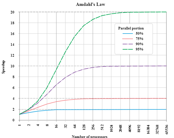
Source: https://en.wikipedia.org/wiki/Amdahl%27s_law#/media/File:AmdahlsLaw.svg

What becomes clear is adding processors only adds so much additional speed, and plateaus pretty quickly. A more dynamic factor is parallelization. Increasing the parallelization from 50% to 75% can increase the speed from 2x speed up to 4x, for example. But the plateau still exists.

What this means for machine learning is, as algorithms become more complex and computationally expensive, throwing more processing power at the issue will have a very limited effect. In the growing world of cloud computing, where an exponential amount of processing power is now actually available, that processing power actually doesn’t help as much as one might want.

Maximizing the amount of parallel operation an algorithm has becomes very important. Avoiding discrete actions will help larger and more complex machine learning algorithms process faster. While the gains through parallelization are theoretically great, in practice they are more difficult to obtain. The current machine learning processes are built on top of existing algorithms and computing structures. These existing structures are often discrete, not built for a world with the current amount of data and algorithm complexity. With these limitations the average person executing a machine learning algorithm is very limited in the amount of parallelization they can implement. It will take experts in these underlying structures rebuilding new building blocks to get greater gains.

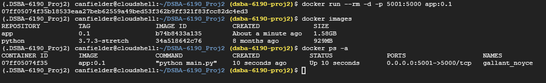
Interactive Lab

Post a screenshot of a lab where you had difficulty with a concept or learned something.

This weeks training was about Docker Containers. I’ve been having issues with correctly defining ports on the Docker Container in order to connect to it. I was able to work through it and figured out I was defining the docker run call incorrectly.