This weeks #TidyTuesday looks at Volcano Eruptions.

Goal: Create an animation visualizing where volcanic eruptions occur.

The complete code and analysis can be found at the following GitHub repo: https://github.com/canfielder/tidytuesday

For the analysis I will use the following libraries.

if (!require(pacman)) {install.packages('pacman')} 
p_load(
  animation, data.table, gganimate, ggthemes, lubridate, maps, mapdata, 
  maptools, rgdal, rgeos, rnaturalearth, tidyverse
)

Import Data

The Tidy Tuesday page for this week outlines the method for loading all of the available data. There are five different datasets, but I’m only using the eruptions data.

eruptions <- readr::read_csv('https://raw.githubusercontent.com/rfordatascience/tidytuesday/master/data/2020/2020-05-12/eruptions.csv')

Processing

There are two data inputs I will need to develop to visualize where volcanic eruptions occur:

1. World Map
2. Volcanic eruption data, with the date of eruption and location (latitude/longitude)

World Map

Most of the worlds volcanic activity occurs around the Pacific Ocean. Therefore, the map I want to use will have the Pacific at the center. Unfortunately, most of the default maps available use the Pacific Ocean as the edge of the map. Additionally, most available maps use something similar to a Mercator projection, which over represents the size of countries closer to the poles. Luckily, I found a blog post which walked through creating a very visually pleasing Eckert IV projection based, Pacific-centered map. I used the code for this map to make my map. Big thanks to the writer of the blog, Valentin.

The first step is to import a world map. For this step I used the rnaturalearth package to import a country based world map. This is of a standard style with the Pacific Ocean on the edges.

sp_worldmap <-  ne_countries(returnclass='sp')

I then performed the following processing on the map to set up being able to shift it so that the Pacific ocean complete, and no longer on the edge of the map.

# shift central/prime meridian towards west - positive values only
shift <- 180+30

# create "split line" to split polygons
WGS84 <- CRS("+proj=longlat +datum=WGS84 +no_defs +ellps=WGS84 +towgs84=0,0,0")

split.line = SpatialLines(list(Lines(list(Line(cbind(180-shift,
                                                     c(-90,90)))),ID="line")),
                          proj4string=WGS84)

# intersecting line with country polygons
line.gInt <- gIntersection(split.line, sp_worldmap)

# create a very thin polygon (buffer) out of the intersecting "split line"
bf <- gBuffer(line.gInt, byid=TRUE, width=0.000001)  

# split country polygons using intersecting thin polygon (buffer)
sp_worldmap.split <- gDifference(sp_worldmap, bf, byid=TRUE)

For aesthetics I also created a bounding box for my map.

# create a bounding box - world extent
b.box <- as(raster::extent(-180, 180, -90, 90), "SpatialPolygons")

# assign CRS to box
proj4string(b.box) <- WGS84

# create graticules/grid lines from box
grid <- gridlines(b.box, 
                  easts  = seq(from=-180, to=180, by=20),
                  norths = seq(from=-90, to=90, by=10))

Now, we shift the map and create a projection.

# give the PORJ.4 string for Eckert IV projection
proj_eckert <- "+proj=eck4 +lon_0=0 +x_0=0 +y_0=0 +ellps=WGS84 +datum=WGS84 +units=m +no_defs" 

# transform bounding box
grid.DT <- data.table(map_data(SpatialLinesDataFrame(sl=grid, 
                                                     data=data.frame(1:length(grid)), 
                                                     match.ID = FALSE)))

# project coordinates
# assign matrix of projected coordinates as two columns in data table
grid.DT[, c("X","Y") := data.table(project(cbind(long, lat), 
                                           proj=proj_eckert))]

# transform split country polygons in a data table that ggplot can use
dt_worldmap <- data.table(map_data(as(sp_worldmap.split, 
                                      "SpatialPolygonsDataFrame")))

# Shift coordinates
dt_worldmap[, long.new := long + shift]
dt_worldmap[, long.new := ifelse(long.new > 180, long.new-360, long.new)]

# project coordinates 
dt_worldmap[, c("X","Y") := data.table(project(cbind(long.new, lat), 
                                               proj=proj_eckert))]

Now we have our spatial data in the right for to create a map with ggplot.

p_map <- ggplot() + 
  
  # add projected countries
  geom_polygon(data = dt_worldmap, 
               aes(x = X, 
                   y = Y, 
                   group = group), 
               colour = "gray90", 
               fill = "gray80", 
               size = 0.75) +

  # add a bounding box (select graticules at edges)
  geom_path(data = grid.DT[(long %in% c(-180,180) & region == "NS")
                           |(long %in% c(-180,180) & lat %in% c(-90,90) 
                             & region == "EW")], 
            aes(x = X, y = Y, group = group), 
            linetype = "solid", colour = "black", size = .3) +
  

  # Ensures that one unit on the x-axis is the same length 
  # as one unit on the y-axis
  coord_equal() + # same as coord_fixed(ratio = 1)
  
  # set empty theme
  theme_void()

p_map

Volcanic Eruption Data

The loaded eruptions dataset contains all the information required. I only need to create the start date of the volcanic eruption for my animation to work. I will calculate the start date using the lubridate package. Then I will select only the required columns for my final eruptions dataset.

df_input <- eruptions %>% 
  mutate(eruption_date = ymd(paste0(start_year,"-",start_month,"-", 
                                    start_day))) %>% 
  select(eruption_date, latitude, longitude)

I also need to convert the latitude and longitude data to match the projection of the map.

# Shift coordinates
df_input <- df_input %>% 
  mutate(long.new = longitude + shift,
         long.new = if_else(long.new > 180, long.new -360, long.new))

# project coordinates 
eruption_proj <- as.data.frame(project(cbind(df_input$long.new, 
                                             df_input$latitude), 
                                       proj=proj_eckert))

# Add projected coordinates back to the input dataframe
df_input <- df_input %>% mutate(long_proj  = eruption_proj$V1,
                            lat_proj = eruption_proj$V2)

Animation

The first step to creating an animation was creating a static image that I was happy with. Once settled, I could then animate over it.

# Establish Custom Theme Values
theme_erupt <- function(){
  theme(
    plot.title = element_text(size = 25),
    plot.subtitle = element_text(size = 20),
    plot.caption = element_text(size = 15),
    plot.margin =  margin(0.5, 0.5, 0.5, 0.5, "cm")
  )
}

# Define Starting Year for Visual
cutoff_year = 1800

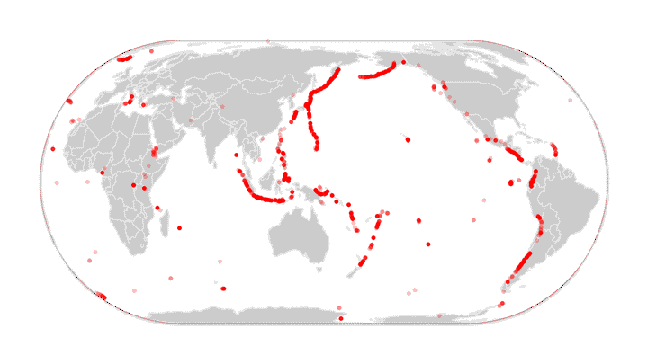
# Map with Volcanic Eruptions
p_static <- p_map + 
  geom_point(data = df_input %>% filter(year(eruption_date) >= cutoff_year),
               mapping = aes(x = long_proj, 
                             y = lat_proj),
             color = '#FF0000', 
             alpha = 0.25,
             size = 2,
             shape = 16) +
  ggtitle(label = "Vocanic Eruptions Around the World",
          subtitle = paste0("From ", cutoff_year," Through Today")) +
  labs(caption = "#TidyTuesday || Created By: Evan Canfield") + 
  theme_erupt()

With the base image set I can then generate and animation using gganimate.

# Define animation
p_animate <- p_static +
  transition_manual(eruption_date, cumulative = TRUE) +
  enter_fade() +
  exit_fade()

# Animation Time (sec)
animation_time = 60

# Set Frames per Second
fps = 10

# Set Sizing Parameters
height_opt = 900
width_opt = 1600
dim_factor = 2

# Generate Gif
gif_world_eruptions <- animate(p_animate,
                               nframes = animation_time * fps,
                               fps = fps,
                               height = height_opt/dim_factor,
                               width = width_opt/dim_factor)

Note: I used the parameter transition_manual as opposed to a time-based transition. This is due to an error I was getting related to using geom_polygons to create the base map. The package gganimate doesn’t play well with polygons. In the future I would try to keep my spatial data in Shapefile form and use coord_sf and other shapefile centric parameters with ggplot.